Basic R • cancR

Overview

The main panel in R consists of four quadrants:
- Script
- Console
- Environment
- Files/plots

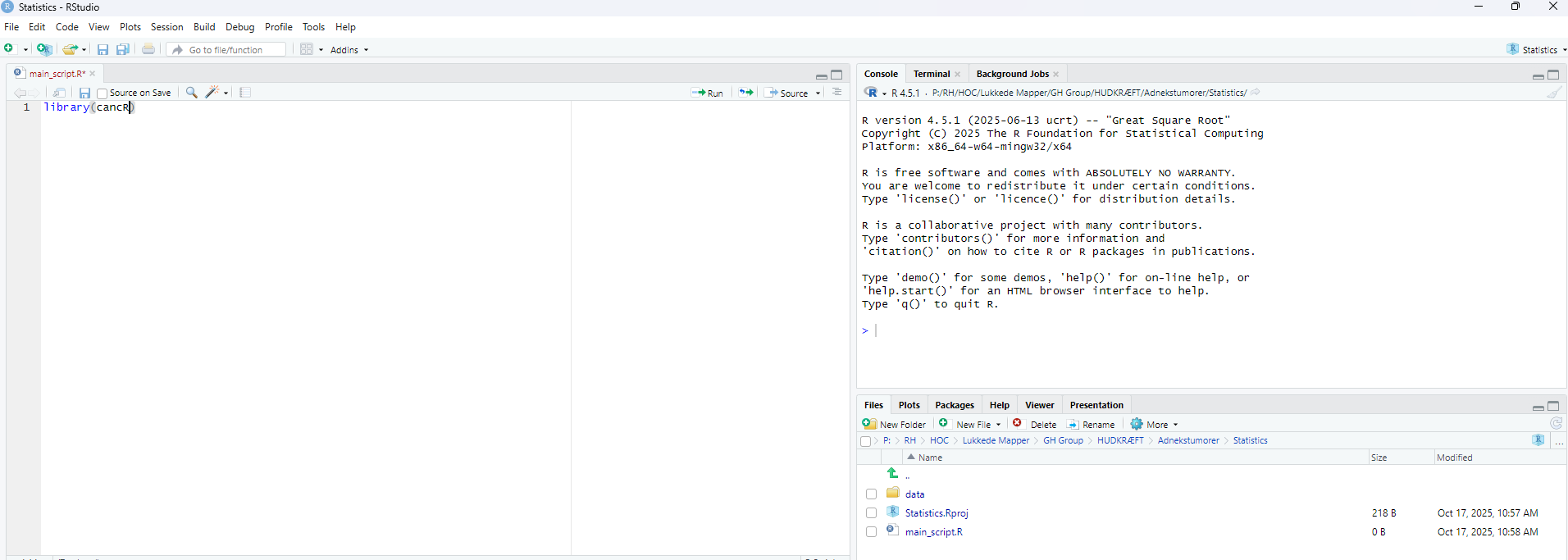
Script

The script is the main working tool. Code in a script is saved and can be reloaded at a later time point. Think of it as a word document or excel sheet in which you work. Ctrl + enter runs a command in the script.

Console

The console has two functions. The first function is that the console prints results from the script and the second is that we can enter commands into the console. An example (press enter to run the command):

2+2
#> [1] 4

We can however browse through previously submitted commands in the console with the arrow up on the keyboard.

The commands entered in the console are temporary and will not be saved for the next R session. Therefore we use the console for commands that we only enter once (e.g. installing packages), quick calculations, minor debugging of code etc.

Environment

The environment is an overview of all loaded data (objects) in R. Currently, nothing is loaded. We can assign a value to an object named x which will now show in the environment.

x <- 1

The arrow indicates that we are assigning something to the environment. We can call this object again, which prints it in the console

x
#> [1] 1

We can also save a data frame

data <- data.frame(x=1, y=2, z=3)

We can view the dataset by clicking on it in the environment. We can also just enter View(data) in the console.

We can also view the data by typing

data
#>   x y z
#> 1 1 2 3

This will print it to the consol. We can also both assign the value and print it simultaneously by adding parentheses around the whole expression

(data <- data.frame(x=1, y=2, z=3))
#>   x y z
#> 1 1 2 3

Files/plots

Under files we can see the current directory and browse through folders. The plot windows opens automatically when we plot something. Here we plot the sequence of numbers 0-10 on both the x and y-axes.

plot(seq(0,10), seq(0,10))

Formats

All values in R have a format for R to process it correctly. The main formats in R are:
- Numerical (numbers)
- Integers (whole numbers)
- Characters (letters/words/text strings)
- Factors (categorical values with specified levels and ordering)
- Dates
- Logicals (True or False)

A common problem is that R functions need specific formats, which entails reformatting to make functions work. Here we define value as the number 1 which is a numeric value. This can be reformatted to the other formats

value <- 1
as.logical(value)
#> [1] TRUE
as.character(value)
#> [1] "1"
as.integer(value)
#> [1] 1
as.Date(value)
#> [1] "1970-01-02"

Logical: Converts 0 to false and everything else to true
Character: Adds " around the value
Integer: Does nothing in this case as the value is already a whole number, but would if the value was 1.5
Date: Converts to 1970-01-02. The time origin in R is 1970-01-01, so the value 1 corresponds to 1970-01-01 + 1 day.

Types of objects

The main types of objects are
- Values
- Vectors
- Dataframes
- Lists
- Functions
- Special objects such as plots, statistical models or other complex objects

Values

These are single values such as a previus example

value <- 1
value
#> [1] 1

Vector

A vector is a string of values. These are collected using a c()

vector <- c(1,2,3,4)
vector
#> [1] 1 2 3 4

Dataframe

A dataframe is a collection of vectors of same lentgh constituting the columns of a dataframe.

v1 <- c(1,2,3,4)
v2 <- c("a", "b", "c", "d")
v3 <- c(1.1, 2.2, 3.3, 4.4)

These three vectors can be combined into one single data frame

df <- data.frame(v1, v2, v3)
df
#>   v1 v2  v3
#> 1  1  a 1.1
#> 2  2  b 2.2
#> 3  3  c 3.3
#> 4  4  d 4.4

Dimensions of a dataframe

We can print the number of rows of a dataframe

nrow(df)
#> [1] 4

And the number of columns

ncol(df)
#> [1] 3

Or together

dim(df)
#> [1] 4 3

Printing values from a dataframe

The names of the dataframe can be extracted with names()

names(df)
#> [1] "v1" "v2" "v3"

An entire column can be extracted with the $ sign

df$v2
#> [1] "a" "b" "c" "d"

Values of the dataframe can also be extracted using square brackets ([]). The syntax here is [rows,columns]. The first row in the third column:

df[1,3]
#> [1] 1.1

Multiple values are collected with c()

df[c(1,2,3), 3]
#> [1] 1.1 2.2 3.3

All rows or columns are selected by leaving the place blank. This prints the entire second column

df[, 2]
#> [1] "a" "b" "c" "d"

Or the entire third row

df[3, ]
#>   v1 v2  v3
#> 3  3  c 3.3

We can also name the columns with a text string

df[, c("v2", "v3")]
#>   v2  v3
#> 1  a 1.1
#> 2  b 2.2
#> 3  c 3.3
#> 4  d 4.4

Creating/modifying values of a dataframe

If we want to create a new variable we assign this to the dataframe using the $

df$new <- "new"
df
#>   v1 v2  v3 new
#> 1  1  a 1.1 new
#> 2  2  b 2.2 new
#> 3  3  c 3.3 new
#> 4  4  d 4.4 new

If we wish to modify an existing variable we use the same procedure

df$v1 <- df$v1 + 5
df
#>   v1 v2  v3 new
#> 1  6  a 1.1 new
#> 2  7  b 2.2 new
#> 3  8  c 3.3 new
#> 4  9  d 4.4 new

Overview of a dataframe

A quick overview (structure) of the content of a dataframe is with str()

str(df)
#> 'data.frame':    4 obs. of  4 variables:
#>  $ v1 : num  6 7 8 9
#>  $ v2 : chr  "a" "b" "c" "d"
#>  $ v3 : num  1.1 2.2 3.3 4.4
#>  $ new: chr  "new" "new" "new" "new"

Here we see the same as above, namely that we have 4 rows (observations) and 4 variables. We also see the names of the variables, the values and the formats (numeric and character).

Lists

Lists are very flexibe objects as we can store different formats in a list as separate elements. Here we make a list containing our dataframe df, our single value valueand our vector vector

list(df, value, vector)
#> [[1]]
#>   v1 v2  v3 new
#> 1  6  a 1.1 new
#> 2  7  b 2.2 new
#> 3  8  c 3.3 new
#> 4  9  d 4.4 new
#> 
#> [[2]]
#> [1] 1
#> 
#> [[3]]
#> [1] 1 2 3 4

The elements are indicating by the [[1]] corresponding to the “first” element etc.

The elements can also be named (for layout we press shift + enter to enter a new line)

(mylist <- list(dataframe = df,
                single_digit = value,
                numbers = vector))
#> $dataframe
#>   v1 v2  v3 new
#> 1  6  a 1.1 new
#> 2  7  b 2.2 new
#> 3  8  c 3.3 new
#> 4  9  d 4.4 new
#> 
#> $single_digit
#> [1] 1
#> 
#> $numbers
#> [1] 1 2 3 4

The elements of a list can be called

mylist["numbers"]
#> $numbers
#> [1] 1 2 3 4

Functions

Functions perform specified commands on a series of arguments. Functions have the syntax:
name(argument 1, argument 2, etc.)

For instance, if we want to take the mean of a vector where we have two arguments:
mean(x, na.rm)

Here x is a vector of values and na.rm indicates whether missing values should be removed in the mean

mean(x=vector, 
     na.rm=T)
#> [1] 2.5

Another example is the plot function from before.
plot(x,y) where x and y are vectors. We could use the vectors from the dataframe df by calling them with $

plot(df$v1, df$v3)